Multi-site Cross-validation of a Flowering Onset Prediction Model for Robinia pseudoacacia

1. Site description and data collection

Bud-burst and flowering date records from observation stations operated by the Korea Meteorological Administration (KMA) were compiled for parameter estimation and validation of the black locust (Robinia pseudoacacia L.) flowering prediction models. Although the overall analytical scope spans from 1973 to 2024, the effective period applied in the analysis was defined independently for each station in accordance with the commencement date of observations and data availability (Table 1, Fig. 1). Daily minimum and maximum air temperature data corresponding to the bud-burst and flowering observation sites were obtained from the Automated Surface Observing System (ASOS) and the KMA seasonal phenological observation records. Both bud-burst and flowering dates were converted to Julian day of year (DOY) for use as model input variables.

Table 1.

Observation periods and statistics of bud-burst and flowering dates (Julian day) for Robinia pseudoacacia at study site

Fig. 1.

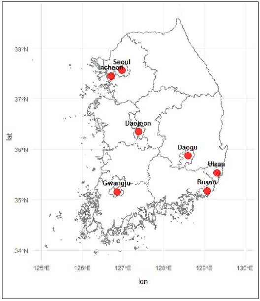
Location map of Korea Meteorological Administration (KMA) ASOS stations representing the study regions for temperature-based modelling of bud-burst and flowering dates of Robinia pseudoacacia. Monitoring sites for bud-burst and blooming dates of Robinia pseudoacacia.

2. Phenological models

1) Chill days model

The Chill Days (CD) model is a process-based model grounded in the dormancy physiology of temperate deciduous trees, distinguishing between two successive phases: endodormancy and ecodormancy (Cesaraccio et al., 2004; Jung et al., 2005; Kim et al., 2021b) (Fig. 2). The model computes chill days (C_d) and anti-chill days (C_a) through five conditional equations based on the relationship between daily minimum and maximum air temperatures and a threshold temperature (T_c) (Cesaraccio et al., 2004, 2005) (Table 2). When the cumulative chill day sum (∑C_d) reaches the chilling requirement (C_R), endodormancy is released. Subsequently, ecodormancy is released and bud-burst is initiated at the point when the cumulative anti-chill day sum (∑C_a) equals |C_d|. The date at which ∑C_a reaches the heat requirement (H_R) following bud-burst is defined as the predicted flowering date (Cesaraccio et al., 2004, 2005; Jung et al., 2005).

Fig. 2.

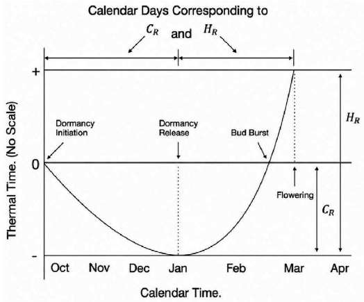
Illustration of thermal time accumulation for dormancy release and flowering. The curve represents the accumulation of chill units until the chilling requirement (CR) is met, followed by the accumulation of heat units until the heating requirement (HR) is reached (Modified from Jung et al., 2005).

Table 2.

Calculation scheme of the chill day (Cd) and anti-chill day (Ca) model (Cesaraccio et al., 2004, 2005)

The threshold temperature (T_c) and chilling requirement (C_R) were constrained to the ranges 5℃≤T_c≤10℃, -300≤C_R≤-70, respectively, based on values reported in the literature (Cesaraccio et al., 2004; Jung et al., 2005; Kim et al., 2013; Chun et al., 2017). The optimal parameter combination was identified via an iterative procedure that minimized the root mean square error (RMSE) between predicted and observed bud-burst dates (Chun et al., 2017). The heat requirement (H_R) was estimated on an annual basis using the selected T_c and C_R following the approach of Jung et al. (2005), and the mean value across years was adopted as the final estimate.

For model implementation, the dormancy onset date was fixed at 1 October of the preceding year (Jung et al., 2005). To prevent overfitting, the full observational dataset was randomly partitioned into training (approximately 60-75%) and validation (approximately 25-40%) subsets. Only splits in which the Wilcoxon rank-sum test indicated no statistically significant difference (p>0.05) in the flowering date distributions between the two subsets were accepted as the final partition (Kim et al., 2021b).

2) Normal Heat Hours (NHH) model

The Normal Heat Hours (NHH) model was developed to overcome the limitation of the linear temperature-development rate relationship assumed by conventional growing degree day (GDD) models, by explicitly accounting for the inhibitory effect of supraoptimal temperatures on developmental rate (Wang and Engel, 1998; Mariani et al., 2013). The model employs a trapezoidal response function defined by four cardinal temperatures, which converts hourly air temperature into NHH values ranging from 0 to 1. NHH equals 0 below the lower cardinal temperature (LC) and above the upper cardinal temperature (UC), NHH equals 1 between the lower optimum temperature (LOC) and the upper optimum temperature (UOC). NHH increases or decreases linearly within the LC-LOC and UOC-UC intervals, respectively (Cola et al., 2017; Alilla et al., 2022).

Since the meteorological dataset used in this study comprises only daily maximum and minimum air temperatures, hourly temperature series were generated by applying the method of Parton and Logan (1981), which employs a sine curve during daytime and an exponential decay curve during nighttime. The potential sunshine duration was calculated from the latitude of each observation site and the solar declination angle.

Model calibration followed the framework of Alilla et al. (2022), with partial modifications to accommodate the use of a single annual flowering date per year in the present study. Whereas the original study calibrated the model through regression analysis using multiple phenological stages (BBCH 51-69), the present study defined the flowering threshold as the median cumulative NHH accumulated up to the observed flowering date across training years, and the date on which this threshold was reached was designated as the predicted flowering date.

Calibration was conducted in two stages. In the first stage, Partial Least Squares (PLS) regression was employed to objectively determine the onset date for NHH accumulation (Luedeling and Gassner, 2012; Luedeling et al., 2013). An 11-day moving average of daily mean temperature was used as the predictor variable to suppress short-term weather noise while preserving the seasonal dormancy signal, and the flowering date (Julian day of year) served as the response variable. The analysis spanned 1 July of the preceding year to 30 June of the target year, covering a full phenological cycle from endodormancy induction to bloom, which allowed the PLS procedure to objectively detect the chilling-to-forcing transition (Luedeling and Gassner, 2012; Luedeling et al., 2013). Based on the resulting Variable Importance in Projection (VIP) scores and standardized regression coefficients, a continuous period in which VIP≥0.8 and rising temperatures exerted a promoting effect on flowering was defined as the forcing phase, and its start date was fixed as the onset date for NHH accumulation.

In the second stage, a grid search was performed over the four cardinal temperature parameters (LC, LOC, UOC, and UC) using the fixed accumulation onset date established in the first stage. The search ranges, following Alilla et al. (2022), were set as LC (0-11°C), LOC (14-19°C), UOC (20-25°C), and UC (26-31°C), with a grid resolution of 1°C and the constraint LC<LOC<UOC<UC enforced throughout (Table 3). For each parameter combination, the median cumulative NHH across training years was defined as the flowering threshold, and the combination yielding the minimum RMSE relative to observed flowering dates was selected as the optimal parameter set. This two-stage procedure provides an independent statistical basis for determining the accumulation onset date, thereby mitigating the risk of overfitting during the grid search process. The training-validation data splitting procedure followed the same Wilcoxon rank-sum test-based protocol applied in the CD model (Kim et al., 2021b).

Table 3.

Parameter ranges tested for model calibration (Modified from Alilla et al., 2022)

3) PhenoFlex model

The PhenoFlex model (Luedeling et al., 2021) is an integrated framework combining the Dynamic Model (DM), which describes chilling accumulation, and the Growing Degree Hours (GDH) model, which describes heat (forcing) accumulation. The model is defined by a total of 12 parameters: six parameters associated with the DM (A₀, A₁, E₀, E₁, T_f and slope), three parameters associated with the GDH model (T_b, T_u and T_c), and three parameters mediating the transition between the two sub-models (y_c, s₁ and z_c). The mathematical algorithms and equations of the PhenoFlex model applied in this study follow those described in Luedeling et al. (2021).

Since the PhenoFlex model requires hourly temperature as input, hourly temperature series were generated from daily maximum and minimum temperatures following the method of Linvill (1990), which simulates daytime temperature using a sine curve and nocturnal cooling using a logarithmic decay function (Luedeling et al., 2021). Approximately 80% of the available years for each city were allocated to calibration, with the remaining 20% reserved for validation. Parameter bounds were adopted from Mojahid et al. (2025) (Table 4). Initial parameter values for the DM parameters were taken from relevant prior studies (Anderson et al., 1985; Fishman et al., 1987a, 1987b; Erez et al., 1989), while those for the transition parameters were set according to the values recommended by Luedeling et al. (2021).

Table 4.

Parameter bounds and initial values used in the Pheno-Flex Enhanced Global Optimization (EGO) based on Mojahid et al. (2025)

To overcome the convergence instability of conventional global optimization approaches arising from inter-parameter scale disparities and susceptibility to local optima, this study adopted the Enhanced Global Optimization method proposed by Mojahid et al. (2025). The method can be summarized by three key features.

First, the activation energy (E) and amplitude (A) parameters of the original DM were replaced with intermediate parameters possessing clear physical interpretations (θ^*, θ_c, π_c and τ), thereby constraining the search space to a physiologically meaningful domain. For each derived parameter combination, Q₁₀ values were computed and restricted to the range 1.5-3.5 to verify biological plausibility.

Second, the MEIGO toolbox (Egea et al., 2014) was employed as the optimization algorithm. MEIGO operates through a structure in which the Enhanced Scatter Search metaheuristic drives global exploration, supplemented by local solvers such as Dynamic Hill Climbing.

Third, the optimization was run independently 10 times (each with 30,000 iterations), after which a weighted ensemble prediction approach was applied to prevent overfitting associated with reliance on a single optimal solution. The final predicted values were derived by weighting the predicted outputs of each run by the Ratio of Performance to Inter-Quartile distance (RPIQ) computed on the validation dataset (Mojahid et al., 2025).

1. Chill days model

The optimal parameters and validation performance of the CD model are presented in Table 5. The threshold temperature (T_c) ranged from 5.0°C (Gwangju) to 8.4°C (Seoul), while the chilling requirement (C_R) ranged from -108 (Seoul) to -199 (Ulsan), with cities located farther south tending to exhibit larger absolute values of C_R. Validation RMSE of the CD model ranged from 1.95 days (Busan) to 4.28 days (Incheon), with a mean RMSE of 2.78 days across the seven cities. The coefficient of determination (R²) ranged from 0.73 (Incheon) to 0.88 (Busan), indicating generally high explanatory power. Notably, the model achieved the best predictive performance in Busan (RMSE=1.95 days, R²=0.88), Ulsan (RMSE=2.06 days, R²=0.84), and Daejeon (RMSE=2.40 days, R²=0.83). In contrast, Incheon exhibited comparatively poor performance, characterized by the highest RMSE (4.28 days) and a pronounced positive bias (Bias=+2.50 days). Positive biases were observed in most cities except Seoul and Busan, suggesting a systematic tendency of the CD model to predict flowering dates later than observed. Seoul (Bias=-0.08 days) and Busan (Bias=-0.40 days), however, showed negligible or marginally early predictions.

Table 5.

Estimated parameters and goodness-of-fit measures for the Chill Days (CD) model across 7 cities

2. Normal Heat Hours (NHH) model

The optimal parameters and validation results of the NHH model are presented in Table 6. The onset date of forcing accumulation (DOY) was earliest in Busan at DOY 45 (mid-February) and latest in Incheon at DOY 92 (early April), revealing an inter-city difference of approximately 47 days. Among the parameters defining the temperature response curve, the optimum temperature range (LOC-UOC) exhibited relatively consistent values across most cities, ranging from 17-19°C to 23-25°C. In contrast, the lower cardinal temperature (LC) showed substantial inter-city variability, spanning from 5°C (Daejeon) to 11°C (Incheon, Ulsan, and Gwangju). The cumulative NHH requirement varied considerably among cities, ranging from 377.7 (Gwangju) to 910.4 (Busan). The notably high NHH requirement observed in Busan is attributable to the low ambient temperatures prevailing during the early forcing period, as the accumulation onset in this city begins as early as DOY 45.

Table 6.

Estimated parameters and goodness-of-fit measures for the Normal Heat Hours (NHH) model across 7 cities

In terms of validation performance, the RMSE of the NHH model ranged from 2.39 days (Busan) to 4.96 days (Gwangju), with a seven-city mean RMSE of 3.46 days. The coefficient of determination (R²) ranged from 0.52 (Gwangju) to 0.82 (Seoul), indicating an overall lower explanatory power compared to the CD model. Satisfactory predictive performance was achieved in Seoul (RMSE=2.43 days, R²=0.82) and Busan (RMSE=2.39 days, R²=0.72); however, markedly diminished accuracy was observed in Gwangju (RMSE=4.96 days, R²=0.52) and Incheon (RMSE=4.29 days, R²=0.53). The bias remained relatively small for most cities, ranging from -1.30 days (Daegu) to +0.86 days (Gwangju), suggesting minimal systematic error. Nevertheless, a moderately pronounced negative bias in Daegu indicated that the model tended to predict flowering dates earlier than the observed values.

3. PhenoFlex model

The estimated 12 parameters and validation performance of the PhenoFlex model are presented in Table 7 and Fig. 3. Among the chilling-related parameters, the critical chilling portion (y_c) was lowest in Seoul (25.83±6.04) and highest in Ulsan (51.64±13.83), suggesting that the chilling requirement is fulfilled with a relatively smaller accumulation in Seoul. The critical forcing accumulation (z_c) ranged from 313.15 (Ulsan) to 444.18 (Daejeon).

Table 7.

Performance evaluation of the PhenoFlex model across seven cities

Fig. 3.

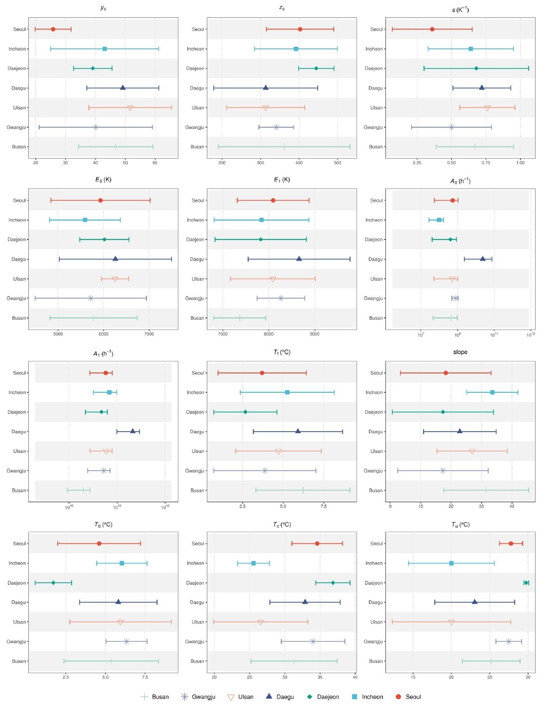
Estimated parameters of the PhenoFlex model across seven cities.

The activation energy parameters, E₀ (5,590.89-6,258.64 K) and E₁ (7,368.14-8,660.04 K), remained at relatively comparable levels across cities. In contrast, the frequency factors (A₀ and A₁) exhibited substantial inter-city variability, spanning orders of magnitude of 10⁸-10¹⁰ and 10¹¹-10¹⁴, respectively. Their associated standard deviations were also large, indicating limited convergence stability in the optimization results. Regarding the forcing-related parameters, the base temperature (T_b) ranged from 1.71°C (Daejeon) to 6.32°C (Gwangju), remaining within a relatively low range across all cities. The upper critical temperature (T_c) ranged from 25.55°C (Incheon) to 36.83°C (Daejeon), and the optimum temperature (T_u) from 20.01°C (Incheon) to 29.76°C (Daejeon), such that the relationship T_b<T_u<T_c held consistently across all cities. Incheon and Ulsan displayed relatively low values of T_c (25.55°C and 26.59°C, respectively) and T_u (20.01°C and 20.02°C, respectively), reflecting a narrow forcing response range. Conversely, Daejeon (T_c=36.83°C, T_u=29.76°C) and Seoul (T_c=34.60°C, T_u=27.77°C) exhibited a considerably wider forcing response range.

The validation results showed that the RMSE of the PhenoFlex model ranged from 2.73 days (Daejeon) to 4.23 days (Seoul), with a seven-city mean RMSE of 3.45 days. The bias remained within ±0.36 days for most cities-the smallest among the three models evaluated-demonstrating well-balanced predictions with minimal systematic error. The coefficient of determination (R²) was reasonably high in Daejeon (0.771), Ulsan (0.746), Gwangju (0.731), and Daegu (0.717), whereas Seoul (0.609) and Busan (0.644) exhibited comparatively lower explanatory power. Notably, Daejeon recorded the best validation performance among all seven cities across all three metrics: RMSE (2.73 days), bias (-0.02 days), and R² (0.771). In contrast, Seoul exhibited the highest RMSE (4.23 days) and the lowest R² (0.609), indicating that the PhenoFlex model was unable to adequately capture the interannual variability in flowering dates in Seoul.

4. Comparison of prediction performance and spatial characteristics among models

Fig. 4 presents scatter plots of observed versus predicted bloom dates for the three models. The CD model (n=291) showed data points clustered around the 1 : 1 line, with an overall RMSE of 3.67 days and R²=0.800. A slight tendency toward overprediction was observed in the early-blooming range (around DOY 110-120) across several cities.

Fig. 4.

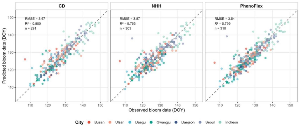
Observed versus predicted flowering dates of Robinia pseudoacacia for the CD, NHH, and PhenoFlex models across seven cities in South Korea. The dashed line represents a perfect match (1 : 1 line) between the observed and predicted dates. Colors indicate the respective cities.

The NHH model (n=303) yielded an RMSE of 3.87 days and R²=0.763, comparable to those of the CD model. A somewhat wider scatter around the 1 : 1 line was apparent in the DOY 120-140 range, which may reflect greater sensitivity of the NHH model to temperature variability during the forcing period.

The PhenoFlex model (n=310) achieved the lowest overall RMSE (3.54 days) with R²=0.799, similar to that of the CD model. Among the three models, PhenoFlex showed the least systematic deviation from the 1 : 1 line, indicating relatively smaller bias across specific bloom date ranges.

Fig. 5 compares the validation results by city and model in a heatmap format. All three models performed well in Daejeon and Ulsan, whereas Incheon exhibited the highest RMSE across all models (CD: 4.28 days, NHH: 4.29 days, PhenoFlex: 3.90 days). The optimal model varied by city: the CD model recorded the lowest RMSE in four cities-Busan (1.95 days), Ulsan (2.06 days), Daejeon (2.40 days), and Gwangju (2.45 days)-while PhenoFlex performed best in Incheon (3.90 days) and Daegu (3.18 days), and NHH in Seoul (2.43 days). The superiority of the CD model was particularly evident in southern cities (Busan, Ulsan, and Gwangju), whereas NHH or PhenoFlex showed relatively better performance in central and northern cities (Seoul and Incheon).

Fig. 5.

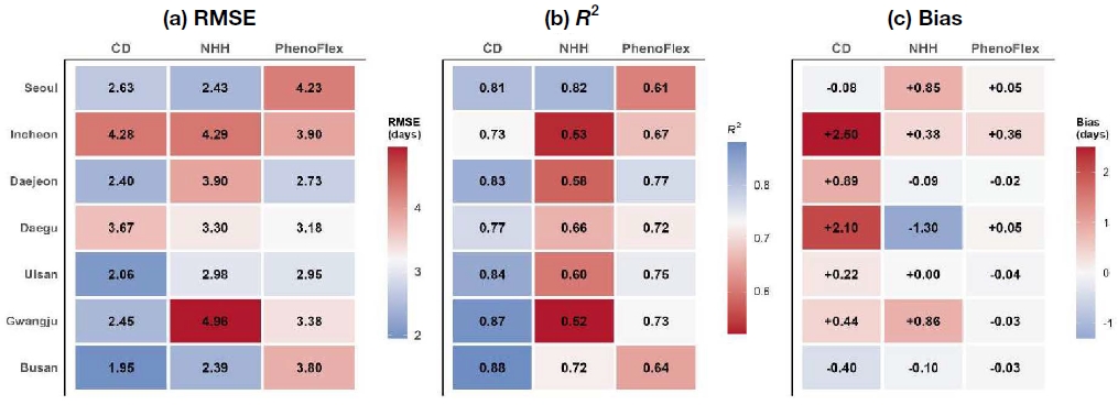
Heatmap comparing the validation performance of the CD, NHH, and PhenoFlex models across seven metropolitan cities: (a) RMSE (days), (b) R2, and (c) Bias (days). Cities on the y-axis are arranged by latitude from north (Seoul) to south (Busan). In panels (a) and (c), blue indicates better performance (lower RMSE or near-zero Bias), while red indicates poorer performance. In panel (b), the color scale is reversed so that blue corresponds to higher R2 values.

The mean RMSE across the seven cities ranked in the order of CD (2.78 days), PhenoFlex (3.45 days), and NHH (3.46 days), and the mean R² followed the same ranking: CD (0.82), PhenoFlex (0.70), and NHH (0.63), indicating that the CD model achieved the highest overall explanatory power. In contrast, PhenoFlex recorded the lowest pooled RMSE, which can be attributed to its more uniform inter-city RMSE range (2.73-4.23 days) compared to that of CD (1.95-4.28 days) and its smaller bias, allowing errors to offset one another when data were aggregated. In terms of bias, the mean absolute bias across the seven cities was 0.08 days for PhenoFlex, markedly smaller than those of CD (0.95 days) and NHH (0.51 days).

1. Model structure and prediction performance

This study compared three process-based models of differing structural complexity under identical conditions, demonstrating that increasing model complexity does not necessarily lead to improved prediction performance. The CD model, with only three parameters, achieved the best city-averaged RMSE and R², whereas the 12-parameter PhenoFlex model was the most stable in terms of pooled RMSE and bias. This indicates that the CD model delivers robust predictive performance against meteorological variability at individual city scales, while PhenoFlex effectively controls systematic bias in region-wide aggregation by continuously simulating the chilling-to-forcing transition.

The finding that an increased number of parameters does not guarantee superior prediction performance is corroborated by previous studies. Yang et al. (2024) reported that a single-parameter GDD model exhibited predictive accuracy comparable to that of nonlinear complex models for rice maturity prediction. Mo et al. (2023) confirmed that simpler models yielded performance similar to that of complex models in a comparison of 17 spring phenology models. García-Gutiérrez and Meza (2023) also reported that a two-parameter model outperformed a ten-parameter model based on the BIC criterion for grapevine. The consistently good performance of the CD model in the present study over long-term datasets spanning 35-52 years is also attributable to the lower risk of overfitting associated with a limited number of parameters.

However, caution is warranted regarding the equifinality problem in complex models such as PhenoFlex, wherein multiple parameter combinations can produce identical outputs (Luo et al., 2009). Luedeling et al. (2021) noted that the 12 parameters of PhenoFlex pose risks of overfitting and derivation of physiologically unrealistic values. Kamimori and Hosomi (2025) reported unrealistically wide effective temperature ranges estimated for grapevine, and Fernandez et al. (2022) demonstrated that thermal response curves varied drastically depending on the temperature range of the calibration data. Therefore, parameters derived from complex models should be interpreted not as absolute physiological values of the trees, but rather as mathematically optimized combinations for achieving optimal predictions under given meteorological conditions.

2. Climatological interpretation of city-specific prediction performance

The spatial heterogeneity in city-specific prediction performance is considered attributable to differences in temperature variability and climatic characteristics among regions. Spring temperature is the most critical factor explaining bloom timing, and a consistent tendency for earlier flowering with rising temperatures has been documented (Pearse et al., 2023; Kim et al., 2025a).

Incheon, which exhibited the highest RMSE across all three models, is a coastal city directly facing the Yellow Sea, where amplified temperature variability driven by land-sea breeze circulation is considered the primary source of prediction error (Cerlini et al., 2022; Guralnick et al., 2024). Temperature fluctuations induced by maritime influence can accumulate errors in thermal time calculations within single-station-based models, a finding supported by the CD model’s bias of +2.50 days-the largest among all cities. In contrast, the consistently good performance of all three models in Daejeon (an inland basin type) and Ulsan (a southeastern coastal type) is interpreted as reflecting the stable interannual variability of winter-to-spring temperatures, which provides favorable conditions for parameter estimation.

The fact that PhenoFlex exhibited its highest RMSE among all seven cities in Seoul suggests that temporal changes in urban heat island intensity associated with rapid urbanization over the past 50 years may have introduced non-stationary temperature-bloom relationships that cannot be captured by the model̓s static parameter framework (Jeong et al., 2011; Meng et al., 2020; Kim et al., 2024).

In terms of latitudinal patterns, the superiority of the CD model was pronounced in southern cities (Busan, Ulsan, Gwangju), whereas NHH or PhenoFlex performed relatively better in central and northern cities (Seoul, Incheon). In southern regions, chilling requirements are fulfilled early and consistently, allowing the sequential structure of the CD model to operate effectively. In central and northern regions, by contrast, greater winter temperature variability and a more gradual chilling-to-forcing transition favor the nonlinear response of NHH or the flexible transition structure of PhenoFlex, which capture these dynamics more adequately.

3. PLS-based forcing start date determination for the NHH model

The PLS-based forcing start date determination applied in this study is significant as an attempt to objectively define the input period for the NHH model. PLS regression can evaluate the influence of temperature at specific periods on phenological responses through VIP scores and regression coefficients, even in daily temperature data characterized by strong autocorrelation (Luedeling and Gassner, 2012), thereby enabling the identification of the chilling-to-forcing transition point (Luedeling et al., 2013). The start dates derived from PLS ranged approximately 47 days, from DOY 45 in Busan to DOY 92 in Incheon, indirectly compensating for the structural limitation of NHH, which lacks an explicit chilling module.

However, the large variation in city-specific performance of the NHH model (Seoul: 2.43 days vs. Gwangju: 4.96 days) reflects the fact that the regional suitability of PLS-determined start dates was not uniform across cities. Furthermore, when the PLS-identified start date is used as a fixed starting point, the inherently gradual chilling-to-forcing transition may not be adequately captured (Luedeling et al., 2013). The lower mean R² of the NHH model compared to those of CD and PhenoFlex is interpreted as partly reflecting this structural sensitivity.

4. Application of PhenoFlex enhanced global optimization

This study represents the first application of the Enhanced Global Optimization (EGO) framework of Mojahid et al. (2025) to black locust (Robinia pseudoacacia) on the Korean Peninsula. By substituting the original parameters with physiologically interpretable intermediate parameters (θ*, θc, πc, τ), the framework sought to simultaneously improve search efficiency and biological plausibility.

Nevertheless, high variability was still observed in the frequency factors (A₀ and A₁). Because A₀ and A₁ are tightly coupled with the activation energies (E₀ and E₁) within the Arrhenius equation, different values can yield identical chilling accumulation through compensatory combinations. In practice, city-specific estimates of A₀ and A₁ varied by several orders of magnitude, whereas E₀ and E₁ remained within a relatively stable range. This constitutes a classic case of equifinality, and field observational data alone have inherent limitations in fully disentangling such compensatory relationships (Fernandez et al., 2022).

To mitigate this issue, RPIQ-based weighted-average prediction was applied to the parameter combinations derived from 10 independent optimization runs (Mojahid et al., 2025). This ensemble approach is considered to have suppressed the risk of overfitting inherent in any single parameter set and contributed to the mean absolute bias of PhenoFlex being the smallest among the three models. However, this remains a statistical remedy for prediction stabilization and does not resolve the physiological uncertainty underlying the chilling accumulation mechanism itself.

5. Comparison with previous studies

The results of this study are broadly consistent with the trends reported in previous research, yet are distinguished by the comparison of three process-based models under identical conditions using long-term, multisite data for black locust.

For the CD model, Kim et al. (2021b) reported that a single-parameter pooled model (SM) across 26 nationwide sites failed to adequately capture inter-regional climatic differences, with the correction coefficient exhibiting a strong positive correlation with mean spring temperature (R²=0.71), resulting in pronounced systematic underestimation in southern regions. In the present study, the base temperature was estimated to be higher in southern cities and lower in central cities, confirming the same directional pattern. The CD RMSE of 3.02-3.22 days reported by Chun et al. (2017) for peach is in good agreement with the mean RMSE of 2.78 days obtained in this study. In contrast, Jeong et al. (2023) reported that the CD model’s dormancy release timing for apple (‘Fuji’) was more than 30 days earlier than that of other models, yielding an RMSE of 8.7 days with poor predictive accuracy, demonstrating that even under the same model structure, performance can vary considerably depending on species-specific chilling requirements and base temperature settings.

Regarding PhenoFlex, Luedeling et al. (2021) reported RMSE values of 3.8-4.0 days with small bias for apple and pear in Germany, which is consistent with the finding in this study that PhenoFlex was the most stable in terms of pooled RMSE and bias. Considered alongside the excellent performance of the DM+GDH combined model (RMSE 1.6-2.0 days) reported by Jeong et al. (2023), model structures that simulate both chilling and forcing nonlinearly may be advantageous for reducing bias across diverse climatic conditions. However, Fernandez et al. (2022) and Mojahid et al. (2025) noted increased RMSE under warm winter conditions and the trade-off between generalizability and regional specificity, respectively, which are consistent with the high variability in frequency factors and the equifinality observed in the present study.

For the NHH model, Alilla et al. (2022) modeled the entire BBCH 51-69 phenological stages using an NHH-based approach in Italy, although their study differed from the present one in that it did not include a chilling module. The highest mean RMSE of NHH in this study is attributable to its structural limitation of not directly simulating the cumulative mechanism of dormancy release, which is also consistent with the finding of Jeong et al. (2023) that models incorporating a chilling phase exhibited greater nationwide applicability than forcing-only models.

6. Limitations and future directions

This study has the following limitations.

First, the PhenoFlex and NHH models estimate hourly temperatures from daily maximum and minimum temperatures, and phenomena such as urban heat islands and land-sea breeze circulations can distort such idealized diurnal temperature curves (Jeong et al., 2011). Furthermore, temperatures recorded by the Automated Synoptic Observing System (ASOS) may not adequately represent the microclimate of forest margins or urban parks where black locust actually grows (De Frenne et al., 2021; Kemppinen et al., 2024). Future studies should incorporate high-resolution gridded meteorological data or in-situ microclimate measurements from forested environments.

Second, all three models use air temperature as the sole driving variable, and other environmental factors potentially involved in flowering-such as soil moisture and photoperiod-are not accounted for (Chuine and Régnière, 2017). Given the projected increase in extreme weather events under climate change, extending the modeling framework to incorporate multiple environmental variables warrants consideration.

Third, to fundamentally reduce the parameter uncertainty inherent in PhenoFlex, temperature-response experiments conducted under controlled environments such as phytotrons should be integrated into the model calibration process (Mojahid et al., 2025). For the NHH model, structural improvements-such as direct coupling with a dynamic chilling module or the implementation of year-specific variable forcing start dates-could be explored to reduce the regional variability in PLS-derived start dates. Moreover, a multi-model ensemble approach that combines the predictions of the three models using city-specific performance-based weights could serve as a viable alternative for enhancing prediction stability.